Children taxa & an effort proxy (SPUE) from the OBIS snapshot

This article shows how to filter OBIS by any WoRMS taxon, at any rank, using only the local OBIS snapshot — no calls to the (heavy) OBIS web services — and how to turn a higher-order taxon into an observation-effort proxy for a presence-only sightings-per-unit-effort (SPUE) indicator. Along the way it produces Table 3 and Figure 4 of the OBIS → H3 → EOV manuscript.

It builds on vignette("h3t"): the same occ_h3 species-level store, plus a baked taxon table (the WoRMS taxonomy) that lets us resolve the descendants of an arbitrary AphiaID.

Why a taxon table?

occ_h3 carries only the six Darwin Core rank columns (phylum … species) plus the species-level aphiaid. That is enough to filter on, say, class = "Aves", but not on a rank that isn’t a column — e.g. Infraorder Cetacea, or an arbitrary clade referenced only by its AphiaID. To support those we walk the full WoRMS hierarchy:

• build_taxon_parquet.R extracts taxonID (= AphiaID), parentNameUsageID, acceptedNameUsageID, scientificName, taxonRank from a WoRMS DarwinCore taxon.txt into a compact taxon.parquet.
• migrate_add_taxon.R bakes that into obis_h3.duckdb (indexed on parentNameUsageID), alongside occ_h3 / idx_h3. The bulk WoRMS download is not a complete cover of the AphiaIDs OBIS carries, so obis_taxon_fill_gaps() closes the gap from the WoRMS REST API (see vignette("eov")).

library(obisindicators)
library(dplyr)
library(ggplot2)

con <- obis_store_connect()   # the store named by OBIS_H3_DUCKDB

Precomputed. The store is not available where this documentation is built, so the database chunks below were run locally by data-raw/precompute_articles.R and their output committed (the tile maps are live). This render used obis_h3_global_v20260728.duckdb, the global store.

Resolve the children of a taxon

obis_taxon_children() returns the seed taxon plus every descendant, at any rank, via a recursive walk of parentNameUsageID. On the full WoRMS table (~1.5 M rows) this resolves in a fraction of a second.

# Infraorder Cetacea = AphiaID 2688 (a rank that is NOT an occ_h3 column)
cet <- obis_taxon_children(2688, con)
nrow(cet)                              # descendant taxa
#> [1] 1665
sort(table(cet$taxonRank), decreasing = TRUE)
#> 
#>     Species       Genus  Subspecies      Family   Subfamily    Subgenus 
#>        1165         231         152          50          29          26 
#> Superfamily  Infraorder     Variety 
#>          10           1           1

# class Bacillariophyceae (diatoms) = 148899: a much broader subtree
dia <- obis_taxon_children(148899, con)
nrow(dia)
#> [1] 71531

The descendant AphiaIDs (cet$taxonID) are exactly the set used to filter occ_h3.aphiaid. obis_taxon_subtree_sql() returns that resolution as a standalone read-only SELECT, handy for the API.

Rank columns vs. subtrees (Table 3)

Why not just filter on the Darwin Core rank columns? Because the rank a name occupies is not stable across taxonomies. A user who filters class = 'Actinopterygii' gets nothing: WoRMS files Actinopterygii as a gigaclass and OBIS’s class column carries Teleostei. class = 'Anthozoa' likewise returns zero (a subphylum in WoRMS; OBIS uses Hexacorallia / Octocorallia). The AphiaID subtree is rank-agnostic and immune to this. calc_rank_vs_subtree() counts each preset group both ways on the base resolution tier of occ_h3.

rv <- calc_rank_vs_subtree(con)
knitr::kable(
  rv |> mutate(across(c(records_rank, records_tree), ~ format(.x, big.mark = ",")),
               ratio = round(ratio, 3)),
  caption = "Records by Darwin Core rank-column filter vs. AphiaID subtree")

Records by Darwin Core rank-column filter vs. AphiaID subtree

label	rank	name	aphiaid	records_rank	species_rank	records_tree	species_tree	ratio
Seabirds	class	Aves	1836	23,686,770	889	23,744,889	891	0.998
Bony fishes	class	Actinopterygii	10194	0	0	45,130,960	16477	0.000
Sharks & rays	class	Elasmobranchii	10193	4,001,773	1144	4,002,304	1145	1.000
Marine mammals	class	Mammalia	1837	4,866,582	170	4,866,582	170	1.000
Sea turtles	order	Testudines	2689	447,735	22	447,743	22	1.000
Corals & anemones	class	Anthozoa	1292	0	0	1,999,366	6258	0.000
Mollusks	phylum	Mollusca	51	10,733,645	34064	10,739,769	34079	0.999
Crustaceans	class	Malacostraca	1071	7,669,820	23968	7,670,453	23987	1.000

long <- bind_rows(
  transmute(rv, label, method = "DwC rank column", records = records_rank),
  transmute(rv, label, method = "AphiaID subtree", records = records_tree))
p <- ggplot(long, aes(x = reorder(label, -records), y = pmax(records, 0.5), fill = method)) +
  geom_col(position = position_dodge(width = .8), width = .7) +
  scale_y_log10(labels = scales::label_comma()) +
  labs(x = NULL, y = "records (log)", fill = NULL,
       title = "Records found by rank-column filter vs AphiaID subtree",
       subtitle = "zero-height bars are groups the rank column cannot express",
       caption = store_label) +
  theme_minimal(base_size = 11) +
  theme(legend.position = "bottom", axis.text.x = element_text(angle = 25, hjust = 1))
p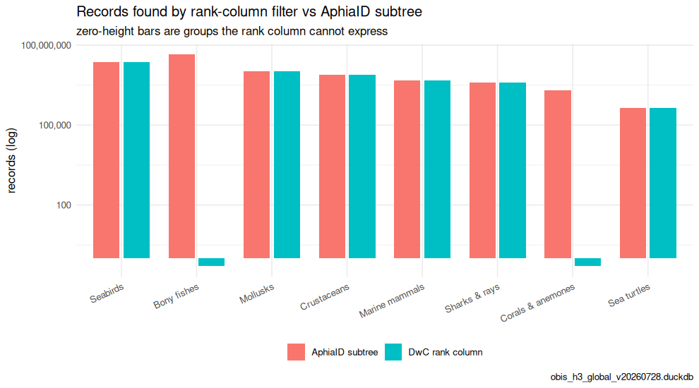

plot of chunk fig-table3

Map a taxon’s records (any rank)

obis_h3t_sql(aphiaid = ...) builds a served tile query that filters occ_h3 to the subtree via a recursive CTE (the h3t validator permits WITH RECURSIVE). obis_h3t_url() base64-encodes it into a tile URL.

sql <- obis_h3t_sql(indicator = "n", aphiaid = 2688)   # # records, all Cetacea
cat(sql)
#> WITH RECURSIVE taxon_tree AS (
#> SELECT taxonID, parentNameUsageID
#> FROM taxon
#> WHERE taxonID IN (2688)
#> UNION ALL
#> SELECT t.taxonID, t.parentNameUsageID
#> FROM taxon t
#> JOIN taxon_tree tt ON t.parentNameUsageID = tt.taxonID
#> WHERE t.parentNameUsageID IS NOT NULL), src AS (
#>   SELECT CAST(h3_cell_to_parent(cell_id, LEAST({{res}}, 7)) AS BIGINT) AS cell_id,
#>          species, SUM(records) AS ni
#>   FROM occ_h3
#>   WHERE res = CASE WHEN LEAST({{res}}, 7) <= 3 THEN 3 WHEN LEAST({{res}}, 7) <= 5 THEN 5 ELSE 7 END
#>     AND aphiaid IN (SELECT taxonID FROM taxon_tree)
#>   GROUP BY 1, 2)
#> SELECT cell_id, SUM(ni) AS value, SUM(ni) AS n FROM src GROUP BY cell_id

url <- obis_h3t_url(
  base_url  = "h3tiles://h3t.marinesensitivity.org/h3t/{z}/{x}/{y}.h3t",
  sql       = sql)

The map below is served live from the deployed tile service (global store):

library(obisindicators)

## Warning: replacing previous import 'h3::compact' by 'purrr::compact' when
## loading 'obisindicators'

library(mapgl)
url <- obis_h3t_url(
  base_url = "h3tiles://h3t.marinesensitivity.org/h3t/{z}/{x}/{y}.h3t",
  sql      = obis_h3t_sql(indicator = "n", aphiaid = 2688))
maplibre(center = c(-40, 20), zoom = 1.5) |>
  add_h3t_source(id = "cet", tiles = url) |>
  add_fill_layer(
    id = "cet_fill", source = "cet", source_layer = "cet",
    fill_color = interpolate(
      column = "value", values = c(1, 1000),
      stops  = c("#3b528b", "#5ec962")))

An effort proxy: sightings per unit effort (SPUE)

A raw record map conflates abundance with observation effort — a hexagon lights up both where a species is common and where people looked hard. When records come from multi-species surveys, a higher-order taxon gives a presence-only proxy for that effort: within the footprint of, say, all Cetacea (the surveys that could have recorded any whale/dolphin), what fraction of records are the target species?

$$\text{SPUE}_{cell} = \frac{\text{records of the target taxon}}{\text{records of the effort taxon}}$$

obis_spue_sql() builds this as a served tile query (two recursive subtrees: numerator = target, denominator = effort). calc_spue() is the pinned R reference (see test-spue-parity.R), and calc_spue_cells() returns the same per-cell table from a store at a fixed resolution.

# target: Tursiops truncatus (common bottlenose dolphin) = 137111
# effort: Infraorder Cetacea = 2688 (its multi-species-survey footprint)
spue_sql <- obis_spue_sql(num_aphiaid = 137111, den_aphiaid = 2688)
cat(spue_sql)
#> WITH RECURSIVE num_tree AS (
#> SELECT taxonID, parentNameUsageID
#> FROM taxon
#> WHERE taxonID IN (137111)
#> UNION ALL
#> SELECT t.taxonID, t.parentNameUsageID
#> FROM taxon t
#> JOIN num_tree tt ON t.parentNameUsageID = tt.taxonID
#> WHERE t.parentNameUsageID IS NOT NULL),
#> den_tree AS (
#> SELECT taxonID, parentNameUsageID
#> FROM taxon
#> WHERE taxonID IN (2688)
#> UNION ALL
#> SELECT t.taxonID, t.parentNameUsageID
#> FROM taxon t
#> JOIN den_tree tt ON t.parentNameUsageID = tt.taxonID
#> WHERE t.parentNameUsageID IS NOT NULL),
#> src AS (
#>   SELECT CAST(h3_cell_to_parent(cell_id, LEAST({{res}}, 7)) AS BIGINT) AS cell_id,
#>          -- COALESCE so an effort cell lacking the target reads 0, not NULL
#>          -- (matches calc_spue(): sum of no records is 0). presence-only:
#>          -- the target was absent *despite* effort here.
#>          COALESCE(SUM(records) FILTER (WHERE aphiaid IN (SELECT taxonID FROM num_tree)), 0) AS n_num,
#>          SUM(records) AS n_den
#>   FROM occ_h3
#>   WHERE res = CASE WHEN LEAST({{res}}, 7) <= 3 THEN 3 WHEN LEAST({{res}}, 7) <= 5 THEN 5 ELSE 7 END
#>     AND aphiaid IN (SELECT taxonID FROM den_tree)
#>   GROUP BY 1)
#> SELECT cell_id,
#>        n_num::DOUBLE / NULLIF(n_den, 0) AS value,
#>        n_den AS n
#> FROM src

library(obisindicators)
library(mapgl)
spue_url <- obis_h3t_url(
  base_url = "h3tiles://h3t.marinesensitivity.org/h3t/{z}/{x}/{y}.h3t",
  sql      = obis_spue_sql(num_aphiaid = 137111, den_aphiaid = 2688))
maplibre(center = c(-40, 20), zoom = 1.5) |>
  add_h3t_source(id = "spue", tiles = spue_url) |>
  add_fill_layer(
    id = "spue_fill", source = "spue", source_layer = "spue",
    fill_color = interpolate(
      column = "value", values = c(0, 1),
      stops  = c("#440154", "#fde725")))

The tooltip n carries the effort count (denominator): a bright cell backed by a large n is a robust SPUE; a bright cell over n = 3 is noise. Choosing the effort taxon is the analyst’s call — the parent class or order is a sensible default, but a survey-defined group (e.g. Cetacea, seabirds) is often better. See vignette("scaling") for how the denominator’s sparsity behaves across H3 resolutions.

SPUE on a map, and against a species distribution model (Fig. 4)

Humpback whale (Megaptera novaeangliae, AphiaID 137092) over all Cetacea. The effort map is the denominator; the SPUE map is masked to cells with at least min_eff effort records.

num_id  <- as.integer(Sys.getenv("SPUE_NUM", "137092"))
den_id  <- as.integer(strsplit(Sys.getenv("SPUE_DEN", "2688"), ",")[[1]])
min_eff <- as.integer(Sys.getenv("SPUE_MIN_EFFORT", "30"))

sp5 <- calc_spue_cells(con, num_id, den_id, res = 5)

p1 <- gmap_cells(sp5, "effort", label = "effort records", trans = "log10") +
  labs(title = "effort (denominator)")
p2 <- gmap_cells(sp5, "spue", label = "SPUE", mask = sp5$effort >= min_eff) +
  labs(title = sprintf("SPUE, effort ≥ %d", min_eff))
p <- patchwork::wrap_plots(p1, p2, ncol = 2) + patchwork::plot_annotation(caption = store_label)
p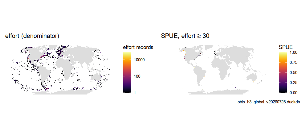

plot of chunk fig4a

Is presence-only SPUE telling us anything about habitat? Compare it with an independent modeled suitability surface for the same species: a GeoTIFF named by SDM_TIF (here the AquaMaps environmental-envelope probability surface for the species, 0–100, from the MarineSensitivity marine atlas — a graded surface; a range mask is constant inside the range and gives no correlation). h3_raster_to_cells() aggregates the raster to the same H3 cells and compare_spue_sdm() reports an effort-gated Spearman correlation plus calibration bins, at each resolution.

sdm_tif <- Sys.getenv("SDM_TIF")
has_sdm <- nzchar(sdm_tif) && file.exists(sdm_tif)
if (!has_sdm) message("set SDM_TIF to run the comparison; skipped")

r  <- terra::rast(sdm_tif)
# crop to the effort footprint (a global 0.05-degree raster is 26M pixels)
bb <- sf::st_bbox(hex_sf(sp5$cell))
r  <- terra::crop(r, terra::ext(bb[["xmin"]] - 1, bb[["xmax"]] + 1, bb[["ymin"]] - 1, bb[["ymax"]] + 1))
res_set <- c(3L, 5L, 7L)
runs <- lapply(res_set, function(rs) {
  spue <- calc_spue_cells(con, num_id, den_id, res = rs)
  sdm  <- h3_raster_to_cells(r, rs, cells = spue$cell)
  list(res = rs, cmp = compare_spue_sdm(spue, sdm, min_effort = min_eff, n_bins = 5L))
})
stats <- bind_rows(lapply(runs, function(x) cbind(res = x$res, x$cmp$stats)))
if (all(is.na(stats$rho)))
  message("rho is NA at every resolution: the surface is constant within the effort footprint ",
          "(a range mask rather than a graded suitability) or too few effort-gated cells overlap it")
knitr::kable(stats |> mutate(across(where(is.numeric), ~ signif(.x, 3))),
             caption = "SPUE vs. modeled suitability by resolution")

SPUE vs. modeled suitability by resolution

res	n_cells	rho	p_value	frac_present
3	2310	0.0087	0.67600	0.714
5	5470	0.1050	0.00000	0.606
7	5980	0.0408	0.00159	0.519

p_rho <- ggplot(stats, aes(x = res, y = rho)) + geom_line() + geom_point(aes(size = n_cells)) +
  scale_x_continuous(breaks = res_set) +
  labs(x = "H3 resolution", y = "Spearman rho (SPUE vs model)", size = "cells",
       title = "Agreement by resolution") + theme_minimal(base_size = 11)
p_cal <- plot_spue_sdm(runs[[2]]$cmp) + labs(title = "Calibration at res 5")
p <- patchwork::wrap_plots(p_rho, p_cal, ncol = 2) + patchwork::plot_annotation(caption = store_label)
p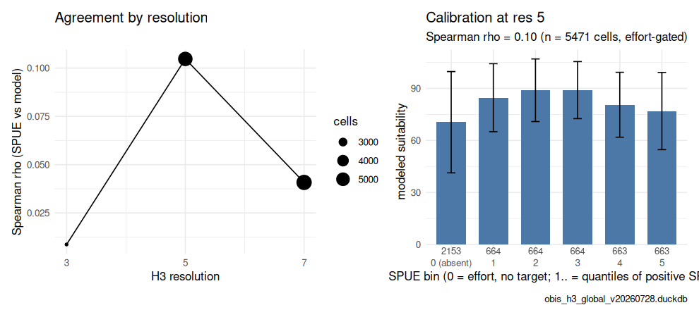

plot of chunk fig4b

sdm5 <- h3_raster_to_cells(r, 5, cells = sp5$cell)
p2 <- patchwork::wrap_plots(
  gmap_cells(sp5, "spue", label = "SPUE", mask = sp5$effort >= min_eff) + labs(title = "observed SPUE"),
  gmap_cells(sdm5, "value", label = "suitability") + labs(title = "modeled suitability"),
  ncol = 2) + patchwork::plot_annotation(caption = store_label)
p2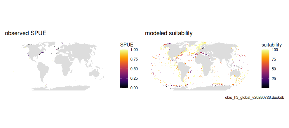

plot of chunk fig4c

On a regional demo store the effort-gated cell count is small and agreement is weak; the point of the comparison is the method — the same effort gate that makes SPUE trustworthy also decides how many cells can be compared at all, and that number falls with resolution (see vignette("scaling")).

DBI::dbDisconnect(con, shutdown = TRUE)