H3 grids and deckgl • obisindicators

Get biological occurrences

Use the 1 million records subsampled from the full OBIS dataset otherwise available at https://obis.org/data/access.

occ <- obisindicators::occ_1M  # global 1M records subset

Create an H3 hexagonal grid

hex_res <- 1  # hex_res 0 is too big to work, all others work
hex <- obisindicators::make_hex_res(hex_res)
# mapview::mapview(hex)  # show the hex grid with h3 IDs 
# === Then assign cell numbers to the occurrence data:
occ <- occ %>% 
  mutate(
    cell = h3::geo_to_h3(
      data.frame(decimalLatitude, decimalLongitude),
      res = hex_res))

Calculate indicators

The following function calculates the number of records, species richness, Simpson index, Shannon index, Hurlbert index (n = 50), and Hill numbers for each cell.

Perform the calculation on species level data:

idx <- obisindicators::calc_indicators(occ)

Add cell geometries to the indicators table (idx):

grid <- hex %>% 
  inner_join(
    idx,
    by = c("hexid" = "cell"))
# you can now visualize with:
# plot(grid["es"])
# mapview::mapview(grid["es"])

Plot maps of indicators

Let’s look at the resulting indicators in map form.

obisindicators::gmap_indicator(
  grid, "es", label = "ES(50)",
  crs="+proj=robin +lon_0=0 +ellps=WGS84 +datum=WGS84 +units=m +no_defs")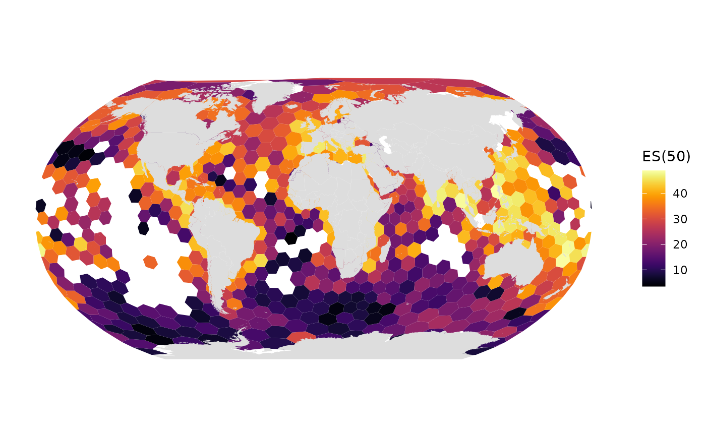

References

`deckgl`

remotes::install_github("crazycapivara/deckgl")
librarian::shelf(
  deckgl, htmlwidgets)

## @knitr h3-cluster-layer
data_url <- paste0(
  "https://raw.githubusercontent.com/uber-common/deck.gl-data/",
  "master/website/sf.h3clusters.json")
# sample_data <- jsonlite::fromJSON(data_url, simplifyDataFrame = FALSE)
sample_data <- data_url

properties <- list(
  stroked = TRUE,
  filled = TRUE,
  extruded = FALSE,
  getHexagons = ~hexIds,
  getFillColor = JS("d => [255, (1 - d.mean / 500) * 255, 0]"),
  getLineColor = c(255, 255, 255),
  lineWidthMinPixels = 2,
  getTooltip = ~mean)

deck <- deckgl(zoom = 10.5, pitch = 20) %>%
  add_h3_cluster_layer(
    data = sample_data, properties = properties) %>%
  add_basemap()

if (interactive())
  deck